CONTENT
Pivot data using Power Query in Power BI
Learn how to transform and pivot data in Power BI for simplified analysis and improved data structure.


Saartje Ly
Data Engineering Intern
Pivot data using Power Query in Power BI
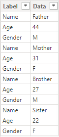
Let's say we have this structure below. It is difficult to analyze, so we want to pivot it.
With Power BI open in your Home tab, click on Transform data.
Now that this data is open in Power Query, we want to add a column for row numbers, to identify each row.
To add a column, navigate to the Add Column tab, then click on Index Column.

Now, we know that each 3 rows are actually 1 row. So, we want another column where the correct row numbers are generated.
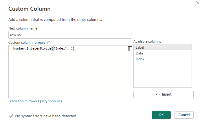
Click on Custom Column
Insert this formula. Here we are saying that we are dividing the Index column by 3. Click OK.

We can now remove the Index column as it has done its job. Right click the header and choose remove.
Now, select Label, go to the Transform tab, and choose Pivot Column.
The names in the Label column will create new columns, automatically merging duplicate names.
Here below we are saying we want the values to come from the Data column. Click on Advanced options, then choose Don't Aggregate from the dropdown to make sure that no summary will be done.

Now we don't need the row no column, it has served its purpose. Right click the header to remove.
Finally select all the columns with ctrl + A, and choose Detect Data Type.

Pivot data using Power Query in Power BI
Let's say we have this structure below. It is difficult to analyze, so we want to pivot it.
With Power BI open in your Home tab, click on Transform data.
Now that this data is open in Power Query, we want to add a column for row numbers, to identify each row.
To add a column, navigate to the Add Column tab, then click on Index Column.
Now, we know that each 3 rows are actually 1 row. So, we want another column where the correct row numbers are generated.
Click on Custom Column
Insert this formula. Here we are saying that we are dividing the Index column by 3. Click OK.
We can now remove the Index column as it has done its job. Right click the header and choose remove.
Now, select Label, go to the Transform tab, and choose Pivot Column.
The names in the Label column will create new columns, automatically merging duplicate names.
Here below we are saying we want the values to come from the Data column. Click on Advanced options, then choose Don't Aggregate from the dropdown to make sure that no summary will be done.
Now we don't need the row no column, it has served its purpose. Right click the header to remove.
Finally select all the columns with ctrl + A, and choose Detect Data Type.
CONTENT
SHARE